
Welcome to The Coding College, where we simplify programming and data science for learners of all levels. In this tutorial, we’ll explore the Binomial Distribution, its significance in statistics, and how to implement it using Python’s NumPy library.
What is a Binomial Distribution?
The Binomial Distribution is a discrete probability distribution that describes the outcome of a fixed number of independent experiments (trials), where each trial has only two possible outcomes: success or failure.
Key Characteristics:
- The number of trials (n) is fixed.
- Each trial has two possible outcomes: success or failure.
- The probability of success (p) is constant for each trial.
- Trials are independent of each other.
Real-Life Examples of Binomial Distribution
- Flipping a coin 10 times and counting the number of heads.
- Checking how many customers out of 100 make a purchase in a store.
- Counting defective items in a batch of products.
Formula for Binomial Probability
The probability of observing k successes in n trials is given by:
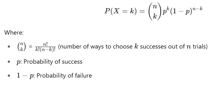
Generating Binomial Distribution in NumPy
Python’s NumPy library provides a function to generate data following a binomial distribution:
Syntax:
numpy.random.binomial(n, p, size=None)n: Number of trials.p: Probability of success.size: Number of random values to generate.
Example 1: Simulating a Binomial Distribution
Generate 10 random values for a process with 5 trials, where the probability of success is 0.6:
import numpy as np

# Generate binomial distribution data
data = np.random.binomial(n=5, p=0.6, size=10)
print(data)
Output (Example):
[3 4 2 5 3 4 3 2 3 5]Example 2: Visualizing a Binomial Distribution
import numpy as np
import matplotlib.pyplot as plt

# Parameters for the binomial distribution
n = 10  # Number of trials
p = 0.5  # Probability of success
size = 1000  # Number of experiments

# Generate data
data = np.random.binomial(n, p, size)

# Plot histogram
plt.hist(data, bins=range(n+2), align='left', rwidth=0.8, color='skyblue')
plt.title('Binomial Distribution (n=10, p=0.5)')
plt.xlabel('Number of Successes')
plt.ylabel('Frequency')
plt.show()
Example 3: Probability of a Specific Outcome
What is the probability of getting exactly 7 successes in 10 trials with a success probability of 0.6?
from math import comb

n = 10
p = 0.6
k = 7

# Calculate binomial probability
prob = comb(n, k) * (p**k) * ((1-p)**(n-k))
print(f"Probability of exactly {k} successes: {prob}")
Output:
Probability of exactly 7 successes: 0.2149908479999999Example 4: Comparing to Other Distributions
The binomial distribution approaches a normal distribution as the number of trials (n) increases.
# Compare binomial distribution with normal approximation
import seaborn as sns

# Parameters
n = 100
p = 0.3
size = 10000

# Generate data
data = np.random.binomial(n, p, size)

# Plot binomial data
sns.histplot(data, kde=True, label='Binomial', color='blue')

# Overlay normal distribution
mean = n * p
std_dev = np.sqrt(n * p * (1 - p))
x = np.linspace(min(data), max(data), 1000)
normal_approx = (1 / (std_dev * np.sqrt(2 * np.pi))) * np.exp(-0.5 * ((x - mean) / std_dev)**2)
plt.plot(x, normal_approx * size * (max(data) - min(data)) / 50, label='Normal Approximation', color='red')

plt.title('Binomial vs. Normal Distribution')
plt.legend()
plt.show()
Applications of Binomial Distribution
- Quality Control: Estimate the probability of defects in a batch.
- Marketing Analysis: Predict the success of campaigns (e.g., conversion rates).
- Medicine: Model outcomes in clinical trials.
- Machine Learning: Analyze classification accuracy.
Summary
The Binomial Distribution is fundamental in statistics, describing processes with binary outcomes. NumPy makes it easy to generate and analyze binomial data, while visualization libraries like Matplotlib and Seaborn allow for effective representation.
For more tutorials and insights, visit The Coding College.