
Welcome to The Coding College, your hub for programming and data science insights! In this article, we will explore the Exponential Distribution, its mathematical foundation, real-world applications, and how to implement it in Python using NumPy.
What is the Exponential Distribution?
The Exponential Distribution is a continuous probability distribution often used to model the time between independent events that occur at a constant average rate. It is closely related to the Poisson Distribution.
Probability Density Function (PDF):
The PDF of the Exponential Distribution is given by:
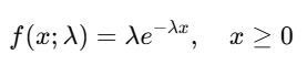
Where:
- x: Random variable (time between events).
- λ\lambda: Rate parameter (1/mean).
Key Characteristics
- Memoryless Property: The probability of an event occurring in the future does not depend on how much time has already passed.
- Mean: 1/λ1/\lambda.
- Variance: 1/λ21/\lambda^2.
Real-Life Applications
- Queueing Theory: Modeling time between customer arrivals.
- Reliability Engineering: Time until a system or component fails.
- Telecommunications: Time between calls in a network.
Exponential Distribution in NumPy
Python’s NumPy library provides a built-in function to generate random numbers from an exponential distribution:
Syntax:
numpy.random.exponential(scale=1.0, size=None)scale: 1/λ1/\lambda (inverse of the rate parameter).size: Output shape (default isNone, which returns a single value).
Example 1: Generating Random Numbers
Scenario: Time between arrivals at a store
import numpy as np

# Generate exponential random numbers
data = np.random.exponential(scale=2.0, size=10)
print("Random times between arrivals:", data)
Output (Example):
[1.02 0.85 3.21 2.13 0.98 4.67 0.42 1.75 2.98 0.25]Example 2: Visualizing Exponential Distribution
import numpy as np
import matplotlib.pyplot as plt

# Generate data
data = np.random.exponential(scale=2.0, size=1000)

# Plot histogram
plt.hist(data, bins=30, color='lightblue', edgecolor='black', density=True)
plt.title('Exponential Distribution (scale=2)')
plt.xlabel('Time between events')
plt.ylabel('Density')
plt.grid(True)
plt.show()
Example 3: Comparing Exponential Distributions
import numpy as np
import matplotlib.pyplot as plt

# Generate data with different scales
data1 = np.random.exponential(scale=1.0, size=1000)
data2 = np.random.exponential(scale=2.0, size=1000)

# Plot histograms
plt.hist(data1, bins=30, alpha=0.5, label='scale=1.0', color='blue', density=True)
plt.hist(data2, bins=30, alpha=0.5, label='scale=2.0', color='orange', density=True)
plt.title('Exponential Distributions with Different Scales')
plt.xlabel('Time between events')
plt.ylabel('Density')
plt.legend()
plt.show()
Real-World Example: Simulating Customer Arrivals
import numpy as np
import matplotlib.pyplot as plt

# Generate random arrival times
lambda_rate = 0.5  # Rate parameter
arrival_times = np.random.exponential(scale=1/lambda_rate, size=100)

# Plot histogram
plt.hist(arrival_times, bins=20, color='purple', edgecolor='black', density=True)
plt.title('Simulated Customer Arrival Times')
plt.xlabel('Time between arrivals')
plt.ylabel('Density')
plt.show()

# Print summary
print("Average time between arrivals:", np.mean(arrival_times))
Exponential vs Poisson Distribution
The Exponential Distribution describes the time between events, while the Poisson Distribution describes the number of events in a fixed interval.
| Aspect | Exponential | Poisson |
|---|---|---|
| Focus | Time between events | Number of events in a fixed time |
| Parameter | Rate parameter (λ\lambda) | Rate parameter (λ\lambda) |
| Relationship | Inter-arrival times in Poisson processes | Events per interval are Poisson-distributed |
Advanced Use Case: Waiting Time Simulation
Scenario: Modeling service time in a call center
import numpy as np
import matplotlib.pyplot as plt

# Parameters
n_calls = 50  # Number of calls
lambda_rate = 0.25  # Average rate of service

# Generate service times
service_times = np.random.exponential(scale=1/lambda_rate, size=n_calls)

# Cumulative waiting time
cumulative_time = np.cumsum(service_times)

# Plot waiting times
plt.plot(cumulative_time, range(1, n_calls + 1), marker='o', linestyle='-', color='teal')
plt.title('Cumulative Waiting Time for Call Center')
plt.xlabel('Time')
plt.ylabel('Number of Calls')
plt.grid(True)
plt.show()
Applications in Machine Learning
- Survival Analysis: Predicting the time until an event occurs (e.g., customer churn).
- Recommendation Systems: Modeling the time between user interactions.
- Traffic Modeling: Predicting inter-arrival times of network packets.
Summary
The Exponential Distribution is an essential tool for modeling time-related data, from queueing systems to failure analysis. Python’s NumPy library makes it easy to simulate and visualize this distribution, helping you gain insights into real-world phenomena.
For more tutorials on coding, statistics, and machine learning, visit The Coding College.