
The perceptron is one of the simplest types of artificial neural networks, and its training process is the foundation for understanding more advanced machine learning models. This article will guide you through the process of training a perceptron, explaining its principles, algorithm, and implementation. For more coding and programming tutorials, visit The Coding College.
How Does a Perceptron Learn?
The perceptron learns by adjusting its weights and bias to minimize the error between its predicted output and the actual output. This is achieved through an iterative process called the perceptron learning algorithm, which uses the concept of error correction.
Steps in Training a Perceptron
- Initialization
- Assign random initial weights (w1,w2,…,wn) and bias (b).
- Set a learning rate (η), typically a small positive value like 0.01 or 0.1.
- Input Data
- Provide a dataset with input features (X) and corresponding labels (y).
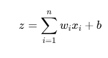
- Weighted Sum
- Calculate the weighted sum (z):
- Activation Function
- Apply a step function to produce the output (y^):

- Error Calculation
- Compute the error (e): e=y−y^
- Weight Update Rule
- Update weights and bias to reduce the error: wi=wi+η⋅e⋅xi b=b+η⋅e
- Repeat
- Repeat steps 3–6 for a set number of epochs or until the error becomes negligible.
Example: Training a Perceptron for an AND Gate
The AND gate is a simple binary classification problem where:
- Inputs: X={[0,0],[0,1],[1,0],[1,1]}
- Labels: y={0,0,0,1}
Python Implementation
import numpy as np

# Step Activation Function
def step_function(z):
    return 1 if z >= 0 else 0

# Perceptron Class
class Perceptron:
    def __init__(self, learning_rate=0.1, epochs=10):
        self.lr = learning_rate
        self.epochs = epochs
        self.weights = None
        self.bias = None

    def fit(self, X, y):
        n_samples, n_features = X.shape
        self.weights = np.zeros(n_features)
        self.bias = 0

        for _ in range(self.epochs):
            for idx, x_i in enumerate(X):
                z = np.dot(x_i, self.weights) + self.bias
                y_pred = step_function(z)
                error = y[idx] - y_pred

                # Update weights and bias
                self.weights += self.lr * error * x_i
                self.bias += self.lr * error

    def predict(self, X):
        z = np.dot(X, self.weights) + self.bias
        return np.array([step_function(i) for i in z])

# Dataset: AND Gate
X = np.array([[0, 0], [0, 1], [1, 0], [1, 1]])
y = np.array([0, 0, 0, 1])

# Train Perceptron
perceptron = Perceptron(learning_rate=0.1, epochs=10)
perceptron.fit(X, y)

# Predictions
predictions = perceptron.predict(X)
print("Predictions:", predictions)
Visualizing Training Progress
Training progress can be visualized by plotting the decision boundary as weights are updated. Tools like Matplotlib can be used to display how the perceptron adapts over epochs.
Challenges in Training Perceptrons
- Linear Separability
- The perceptron only works for linearly separable data. For example, it cannot classify XOR gate inputs.
- Convergence
- The perceptron converges only when the data is linearly separable. Otherwise, it fails to find a solution.
- Learning Rate
- Selecting an appropriate learning rate is crucial to ensure smooth and efficient convergence.
Beyond Perceptrons
When the perceptron model’s limitations are encountered, more advanced models like multi-layer perceptrons (MLPs) or deep learning architectures are used to handle non-linear and complex patterns.