
Welcome to The Coding College, your trusted source for learning all things related to data science. In this post, we will walk you through a practical linear regression case. Linear regression is one of the most widely used techniques in data science for predicting a continuous dependent variable based on one or more independent variables. Through this example, you’ll gain a deeper understanding of how linear regression works and how it can be applied in real-world scenarios.
What Is Linear Regression?
Linear regression is a statistical method used to model the relationship between a dependent variable and one or more independent variables by fitting a linear equation to the observed data. The goal is to find the line (or hyperplane, in the case of multiple predictors) that best represents the relationship between the variables.
The equation for a simple linear regression is:
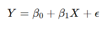
Where:
- Y is the dependent variable (the value you want to predict),
- X is the independent variable (the predictor),
- β0\beta_0 is the intercept (the value of YY when X=0X = 0),
- β1\beta_1 is the coefficient of the independent variable, and
- ϵ\epsilon is the error term (the difference between the actual and predicted values).
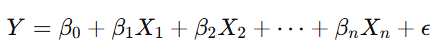
For multiple linear regression, where more than one independent variable is involved, the equation becomes:
Example: Linear Regression Case Study
Let’s go through a simple linear regression case study to demonstrate how linear regression can be applied to predict a real-world outcome. For this example, we’ll predict house prices based on two independent variables: square footage and number of rooms.
The Dataset
We have the following dataset for a few houses:
| House | Square Footage (X1) | Number of Rooms (X2) | Price (Y) |
|---|---|---|---|
| 1 | 1500 | 3 | 300,000 |
| 2 | 1800 | 4 | 350,000 |
| 3 | 2400 | 4 | 400,000 |
| 4 | 2200 | 5 | 380,000 |
| 5 | 2700 | 5 | 450,000 |
In this case, the goal is to predict the price of a house (Y) based on the square footage (X1) and number of rooms (X2). This is a multiple linear regression problem because we have two predictors (X1 and X2).
Step 1: Visualizing the Data
Before we start building the model, it’s helpful to visualize the data to understand the relationships. You can plot scatter plots of the dependent variable (Price) against each independent variable (Square Footage and Number of Rooms).
- Scatter plot of Square Footage vs. Price: This plot will show if there is a linear relationship between the size of the house and its price.
- Scatter plot of Number of Rooms vs. Price: This plot will show how the number of rooms influences the house price.
Step 2: Fitting the Linear Regression Model
We can use the Ordinary Least Squares (OLS) method to fit a linear regression model. The goal is to estimate the coefficients (β0\beta_0, β1\beta_1, and β2\beta_2) that minimize the sum of the squared errors.
Using Python’s scikit-learn library, we can perform the regression and calculate the coefficients.
import numpy as np
import pandas as pd
from sklearn.linear_model import LinearRegression

# Define the dataset
data = {
    'Square Footage': [1500, 1800, 2400, 2200, 2700],
    'Number of Rooms': [3, 4, 4, 5, 5],
    'Price': [300000, 350000, 400000, 380000, 450000]
}

df = pd.DataFrame(data)

# Independent variables (X)
X = df[['Square Footage', 'Number of Rooms']]

# Dependent variable (Y)
Y = df['Price']

# Initialize and fit the model
model = LinearRegression()
model.fit(X, Y)

# Output the coefficients and intercept
print(f"Intercept (β0): {model.intercept_}")
print(f"Coefficients (β1, β2): {model.coef_}")
Step 3: Interpreting the Model Output
Suppose the output of the regression model is:
- Intercept (β0): 100,000
- Coefficient for Square Footage (β1): 150
- Coefficient for Number of Rooms (β2): 20,000
The equation for the regression line is: Price=100,000+(150×Square Footage)+(20,000×Number of Rooms)\text{Price} = 100,000 + (150 \times \text{Square Footage}) + (20,000 \times \text{Number of Rooms})
This means that for each additional square foot, the price increases by $150, and for each additional room, the price increases by $20,000.
Step 4: Making Predictions
Using the fitted model, you can now predict the price of a new house. Let’s predict the price for a house with:
- 2200 square feet and 4 rooms.
# New data for prediction
new_data = np.array([[2200, 4]])

# Predict the price
predicted_price = model.predict(new_data)
print(f"Predicted Price: ${predicted_price[0]:,.2f}")
Step 5: Evaluating the Model
To evaluate the performance of the regression model, you can look at the R-squared value. This tells you how well the model explains the variance in the dependent variable (house price). A higher R-squared indicates that the model has a good fit.
You can also check other metrics like Mean Absolute Error (MAE) or Root Mean Squared Error (RMSE) for a more detailed evaluation.
from sklearn.metrics import mean_squared_error, r2_score

# Predicting the prices for the entire dataset
predictions = model.predict(X)

# Calculating the R-squared value
r2 = r2_score(Y, predictions)
print(f"R-squared: {r2:.2f}")
Step 6: Improving the Model
In practice, models can often be improved by adding more features, transforming variables, or using advanced regression techniques like ridge regression or lasso regression to handle multicollinearity and overfitting.
Conclusion
In this linear regression case, we demonstrated how to predict house prices based on square footage and number of rooms using a multiple linear regression model. By understanding the relationship between the predictors and the target variable, we can make informed predictions and evaluate the performance of the model.
At The Coding College, we provide in-depth content to help you master data science concepts. By understanding the steps involved in building and evaluating a linear regression model, you can apply this knowledge to a variety of real-world problems in data science.