
Welcome to The Coding College, your go-to resource for learning coding and data science concepts! In this article, we’ll explore the Logistic Distribution, its mathematical properties, applications, and how to work with it in Python.
What is Logistic Distribution?
The Logistic Distribution is a continuous probability distribution often used in statistics, machine learning, and data science. It is symmetric, similar to the Normal Distribution, but has heavier tails, which makes it more sensitive to outliers.
Probability Density Function (PDF):
The PDF of a Logistic Distribution is given by:
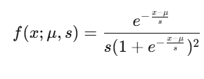
Where:
- μ: Location parameter (mean).
- s: Scale parameter (related to standard deviation).
- x: Random variable.
Key Properties
- Symmetry: The distribution is symmetric around the mean μ\mu.
- Heavy Tails: Compared to the normal distribution, the logistic distribution assigns more probability to extreme values.
- Applications: Used in logistic regression, machine learning classification problems, and modeling growth processes.
Real-Life Applications
- Machine Learning: Activation function in logistic regression and neural networks.
- Economics: Modeling price elasticity of demand.
- Biostatistics: Modeling growth rates (e.g., population growth).
Logistic Distribution in NumPy
Python’s NumPy library provides a straightforward way to generate data from a logistic distribution:
Syntax:
numpy.random.logistic(loc=0.0, scale=1.0, size=None)loc: Location parameter (μ\mu).scale: Scale parameter (ss).size: Output shape (default isNone, which returns a single value).
Example 1: Generate Logistic Random Numbers
import numpy as np

# Generate logistic distribution data
data = np.random.logistic(loc=0, scale=1, size=10)
print("Logistic random numbers:", data)
Output (Example):
[0.84 -0.31 1.24 0.52 -0.71 2.03 -0.15 -0.49 0.33 1.72]Example 2: Visualizing Logistic Distribution
import numpy as np
import matplotlib.pyplot as plt

# Generate data
data = np.random.logistic(loc=0, scale=1, size=1000)

# Plot histogram
plt.hist(data, bins=30, color='skyblue', edgecolor='black', density=True)
plt.title('Logistic Distribution (loc=0, scale=1)')
plt.xlabel('Value')
plt.ylabel('Frequency')
plt.show()
Example 3: Comparing Logistic and Normal Distributions
import numpy as np
import matplotlib.pyplot as plt
from scipy.stats import norm

# Generate logistic and normal data
logistic_data = np.random.logistic(loc=0, scale=1, size=1000)
normal_data = np.random.normal(loc=0, scale=1, size=1000)

# Plot histograms
plt.hist(logistic_data, bins=30, alpha=0.5, label='Logistic', color='blue', density=True)
plt.hist(normal_data, bins=30, alpha=0.5, label='Normal', color='orange', density=True)
plt.title('Logistic vs Normal Distribution')
plt.xlabel('Value')
plt.ylabel('Density')
plt.legend()
plt.show()
Logistic Growth Model
The logistic distribution is often used in modeling growth, such as population growth, where growth starts exponentially but slows as it reaches a carrying capacity.
Logistic Growth Function:
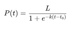
Where:
- P(t): Population at time tt.
- LL Carrying capacity (maximum population).
- k: Growth rate.
- t0: Time of maximum growth.
Example 4: Simulating Logistic Growth
import numpy as np
import matplotlib.pyplot as plt

# Parameters
L = 100  # Carrying capacity
k = 0.1  # Growth rate
t0 = 50  # Time of maximum growth
t = np.linspace(0, 100, 500)  # Time values

# Logistic growth function
P = L / (1 + np.exp(-k * (t - t0)))

# Plot logistic growth
plt.plot(t, P, color='green')
plt.title('Logistic Growth Model')
plt.xlabel('Time')
plt.ylabel('Population')
plt.grid(True)
plt.show()
Key Differences: Logistic vs Normal Distribution
| Aspect | Logistic | Normal |
|---|---|---|
| Shape | Bell-shaped | Bell-shaped |
| Tails | Heavier tails | Lighter tails |
| Symmetry | Symmetric | Symmetric |
| Applications | Growth modeling, ML | General statistics |
Applications of Logistic Distribution in Machine Learning
- Logistic Regression: Used to model binary outcomes (0 or 1).
- Neural Networks: Logistic function as an activation function (sigmoid).
- Class Probabilities: Predicting probabilities in classification problems.
Summary
The Logistic Distribution is an essential concept in statistics and machine learning. It provides a foundation for understanding growth models, classification problems, and probability theory. With Python’s NumPy, you can easily generate and visualize logistic distribution data, making it a powerful tool for data analysis and modeling.
For more insightful tutorials and examples, visit The Coding College.