
Welcome to The Coding College, your go-to resource for simplifying data science and programming concepts! In this guide, we’ll explore the Pareto Distribution, its significance, properties, applications, and how to implement it in Python using NumPy.
What is the Pareto Distribution?
The Pareto Distribution, also known as the Power Law Distribution, is a continuous probability distribution that describes phenomena where a small proportion of causes contributes to the majority of effects. This is often referred to as the 80/20 rule: 80% of outcomes come from 20% of causes.
Probability Density Function (PDF):
The PDF of the Pareto Distribution is given by:
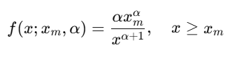
Where:
- xm: The minimum value (scale parameter, x>0).
- α\alpha: The shape parameter (>0).
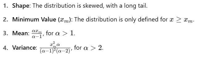
Key Characteristics
Real-Life Applications
- Wealth Distribution: A small percentage of individuals hold most of the wealth.
- Natural Phenomena: Earthquake magnitudes, city populations, and forest fire sizes.
- Business: Product sales where a few products generate most of the revenue.
- Internet Traffic: A small percentage of users generate most of the traffic.
Pareto Distribution in NumPy
Python’s NumPy library provides a function to generate random samples from the Pareto distribution:
Syntax:
numpy.random.pareto(a, size=None)a: Shape parameter (α\alpha).size: Output shape (default isNone, which returns a single value).
Example 1: Generating Random Numbers
Scenario: Simulate wealth distribution
import numpy as np

# Generate Pareto random numbers
alpha = 3  # Shape parameter
data = np.random.pareto(a=alpha, size=10) + 1  # Add 1 to include the minimum value
print("Random samples from Pareto distribution:", data)
Output (Example):
[1.54 1.21 1.13 1.75 1.32 1.89 1.05 1.67 1.23 1.45]Example 2: Visualizing the Pareto Distribution
import numpy as np
import matplotlib.pyplot as plt

# Generate data
alpha = 2.0
data = np.random.pareto(a=alpha, size=1000) + 1  # Add 1 for the scale

# Plot histogram
plt.hist(data, bins=50, color='skyblue', edgecolor='black', density=True)
plt.title('Pareto Distribution (α=2)')
plt.xlabel('Value')
plt.ylabel('Density')
plt.grid(True)
plt.show()
Example 3: Comparing Pareto Distributions
Scenario: Analyze the effect of the shape parameter
import numpy as np
import matplotlib.pyplot as plt

# Generate data with different shape parameters
data1 = np.random.pareto(a=1.5, size=1000) + 1
data2 = np.random.pareto(a=3.0, size=1000) + 1
data3 = np.random.pareto(a=5.0, size=1000) + 1

# Plot histograms
plt.hist(data1, bins=50, alpha=0.5, label='α=1.5', density=True, color='blue')
plt.hist(data2, bins=50, alpha=0.5, label='α=3.0', density=True, color='orange')
plt.hist(data3, bins=50, alpha=0.5, label='α=5.0', density=True, color='green')

plt.title('Pareto Distributions with Different Shape Parameters')
plt.xlabel('Value')
plt.ylabel('Density')
plt.legend()
plt.grid(True)
plt.show()
Example 4: Transforming the Pareto Distribution
You can customize the Pareto Distribution by multiplying by a scale factor (xmx_m):
import numpy as np

# Shape and scale parameters
alpha = 2.5
x_m = 2  # Minimum value (scale parameter)

# Generate Pareto random numbers
data = (np.random.pareto(a=alpha, size=1000) + 1) * x_m

# Print sample statistics
print("Mean:", np.mean(data))
print("Variance:", np.var(data))
Properties of the Pareto Distribution
| Property | Description |
|---|---|
| Shape Parameter (α\alpha) | Determines the “heaviness” of the tail. |
| Scale Parameter (xmx_m) | Minimum value; shifts the distribution. |
| Mean | Finite for α>1\alpha > 1. |
| Variance | Finite for α>2\alpha > 2. |
| Applications | Wealth distribution, internet traffic, and natural phenomena. |
Pareto vs Other Distributions
| Aspect | Pareto | Exponential | Normal |
|---|---|---|---|
| Type | Continuous | Continuous | Continuous |
| Focus | Skewed with a long tail | Time between events | Symmetric data |
| Applications | Wealth, natural phenomena | Queueing models | General data analysis |
Summary
The Pareto Distribution is a versatile tool for modeling power-law phenomena in various fields