
Welcome to The Coding College, where we simplify coding and programming concepts for all learners! In this article, we explore the Zipf Distribution, its unique properties, real-world applications, and how to implement it in Python using NumPy.
What is the Zipf Distribution?
The Zipf Distribution is a discrete probability distribution that models data where the frequency of an event is inversely proportional to its rank in a frequency table. This distribution is closely associated with Zipf’s Law, which is often observed in linguistics, social sciences, and information systems.
Probability Mass Function (PMF):
The PMF of the Zipf Distribution is given by:
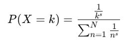
Where:
- k: Rank of the event (k≥1).
- s: Skew parameter (s>0).
- N: Total number of ranks.
Key Characteristics
- Rank-Frequency Rule: Higher-ranked items occur less frequently.
- Skewness: Controlled by the skew parameter ss. Higher ss increases the dominance of top-ranked items.
- Discrete Distribution: Values are integers starting from 1.
Real-Life Applications
- Linguistics: Word frequency in natural languages.
- City Populations: Size distribution of cities in a region.
- Web Traffic: Page views or click-through rates.
- Economics: Income rankings and wealth distribution.
- Information Systems: Query frequency in search engines.
Zipf Distribution in NumPy
Python’s NumPy library provides a function to generate random samples from the Zipf distribution:
Syntax:
numpy.random.zipf(a, size=None)a: Skew parameter (ss).size: Output shape (default isNone, which returns a single value).
Example 1: Generating Random Numbers
Scenario: Simulate word frequency in a text corpus
import numpy as np

# Generate Zipf random numbers
skew = 2.0  # Skew parameter
data = np.random.zipf(a=skew, size=10)
print("Random samples from Zipf Distribution:", data)
Output (Example):
[1 1 2 1 1 3 1 1 1 2]Example 2: Visualizing the Zipf Distribution
import numpy as np
import matplotlib.pyplot as plt

# Generate data
skew = 1.5
data = np.random.zipf(a=skew, size=10000)

# Count occurrences of ranks
unique, counts = np.unique(data, return_counts=True)

# Plot rank vs frequency
plt.loglog(unique, counts, marker="o", linestyle="none")
plt.title('Zipf Distribution (s=1.5)')
plt.xlabel('Rank')
plt.ylabel('Frequency')
plt.grid(True, which="both", linestyle="--", linewidth=0.5)
plt.show()
Example 3: Comparing Zipf Distributions
Scenario: Analyze the effect of the skew parameter
import numpy as np
import matplotlib.pyplot as plt

# Generate data with different skew parameters
data1 = np.random.zipf(a=1.2, size=10000)
data2 = np.random.zipf(a=2.0, size=10000)
data3 = np.random.zipf(a=3.0, size=10000)

# Count occurrences of ranks
unique1, counts1 = np.unique(data1, return_counts=True)
unique2, counts2 = np.unique(data2, return_counts=True)
unique3, counts3 = np.unique(data3, return_counts=True)

# Plot data
plt.loglog(unique1, counts1, label='s=1.2', marker="o", linestyle="none")
plt.loglog(unique2, counts2, label='s=2.0', marker="o", linestyle="none")
plt.loglog(unique3, counts3, label='s=3.0', marker="o", linestyle="none")

plt.title('Zipf Distribution with Different Skew Parameters')
plt.xlabel('Rank')
plt.ylabel('Frequency')
plt.legend()
plt.grid(True, which="both", linestyle="--", linewidth=0.5)
plt.show()
Example 4: Modeling Word Frequencies
Scenario: Analyze the frequency of words in a synthetic dataset
import numpy as np
import matplotlib.pyplot as plt

# Generate Zipf random numbers
data = np.random.zipf(a=1.5, size=10000)

# Count frequencies
unique, counts = np.unique(data, return_counts=True)

# Display top 10 words
top_words = list(zip(unique[:10], counts[:10]))
print("Top 10 words by rank and frequency:", top_words)

# Plot histogram
plt.bar(unique[:10], counts[:10], color='skyblue', edgecolor='black')
plt.title('Top 10 Words by Rank')
plt.xlabel('Rank')
plt.ylabel('Frequency')
plt.grid(axis='y')
plt.show()
Properties of the Zipf Distribution
| Property | Description |
|---|---|
| Skew Parameter (ss) | Determines the steepness of the rank-frequency curve. |
| Discrete Nature | Values are integers starting from 1. |
| Applications | Linguistics, web traffic, city populations, and income distribution. |
Zipf vs Other Distributions
| Aspect | Zipf | Pareto | Normal |
|---|---|---|---|
| Type | Discrete | Continuous | Continuous |
| Focus | Rank-based data | Skewed, power-law data | Symmetric data |
| Applications | Word frequency, page ranks | Wealth distribution | General data analysis |
Summary
The Zipf Distribution is a fascinating model for rank-based systems, with applications in various fields like linguistics, information systems, and economics. Python’s NumPy library makes it simple to simulate, analyze, and visualize this distribution.
For more in-depth programming tutorials, visit The Coding College.